We've got a new radio design, originally from Dick Smith Electronics, I believe. It uses three pennies as solder pads, and is the same old basic MK484 receiver.
I designed this for a kitbuilding activity at the 2019 Bloomington, Indiana hamfest. Most of the parts are available from your favorite electronics hobby store, or online. Lots of them are available from Mike's Electronic Parts.
The radio features a unique plug-in on/off switch. The positive wire for the battery connects to the circuit when a mono plug is inserted into the stereo jack, shorting the collar and sleeve contacts together.
The dial for the capacitor is on a sheet. Print it out on cardstock and punch/cut it out. It's useful for many projects that use a polyvaricon.
Saturday, September 28, 2019
Wednesday, June 19, 2019
Monday, March 07, 2016
MATLAB Smith Charts
Last time, I posted a procedure for creating Smith charts by hand.
This time, I’d like to continue the process by showing my procedure for using Matlab® or GNU Octave to create these charts.
I should note that Matlab® already has a “smithchart” function, that does a pretty good job. But if you’d like to customize the chart or do it in GNU Octave, this process might be better. Matlab®’s function will plot a reflection coefficient for you, while the script presented here does not.
Matlab® or Octave, the smithchart function or script doesn’t do the \(Z\) to \(\Gamma\) conversion for you. The function simply draws the circles on in Cartesian coordinates. You still have to convert an impedance to a reflection coefficient.
$$\Gamma = \frac{Z - Z_0}{Z + Z_0}$$
where is the basis impedance for the chart.
The real and imaginary part of the reflection coefficient will be the and coordinates that to plot.
We will not plot complete circles for all resistances. This will lead to a very cluttered chart on the right hand side. Instead we will start and stop them at strategic locations on the chart.
The complex impedance can be broken down into
$$Z=A+jB$
Where is the resistance and is the reactance. In a Smith Chart, all impedances are normalized to one. The reflection coefficients for the circles become
This time, I’d like to continue the process by showing my procedure for using Matlab® or GNU Octave to create these charts.
I should note that Matlab® already has a “smithchart” function, that does a pretty good job. But if you’d like to customize the chart or do it in GNU Octave, this process might be better. Matlab®’s function will plot a reflection coefficient for you, while the script presented here does not.
Matlab® or Octave, the smithchart function or script doesn’t do the \(Z\) to \(\Gamma\) conversion for you. The function simply draws the circles on in Cartesian coordinates. You still have to convert an impedance to a reflection coefficient.
$$\Gamma = \frac{Z - Z_0}{Z + Z_0}$$
where is the basis impedance for the chart.
The real and imaginary part of the reflection coefficient will be the and coordinates that to plot.
Zero reactance line
The zero reactance line is the axis. We just draw a line from -1 to 1.x = linspace (-1, 1, 256);
y = zeros (1, length (x));
plot (x, y,'k');
% We don't show the axis, but we need to scale it.
axis ([-1.15, 1.15, -1.15, 1.15]);
axis off;
hold on |
| Zero Reactance Line |
Resistance Circles
We will not plot complete circles for all resistances. This will lead to a very cluttered chart on the right hand side. Instead we will start and stop them at strategic locations on the chart.
The complex impedance can be broken down into
$$Z=A+jB$
Where is the resistance and is the reactance. In a Smith Chart, all impedances are normalized to one. The reflection coefficients for the circles become
A = [.2 .5 1 2]; Blim = [1 2 5 2];

for idx = 1:length(A);
    B = linspace (-Blim(idx), Blim(idx), 256);
    rho = (A(idx)^2 + B.^2 - 1 + 2i * B) ./ ...
      ((A(idx) + 1).^2 + B.^2);

    plot (rho, 'k');
end
 |
| Resistance Circles |
Some resistances can have full circles, namely, the -, -, and circles. However, we will never be able to complete the circles using the technique above. The right hand side of the chart is infinity.
Instead, we just make Cartesian circles at those points. It’s easier and saves memory.
theta = linspace (0, 2 * pi, 256); A = [0 5 10];

for idx = 1:length (A)
    cx = A(idx) ./ (A(idx) + 1);
    rx = 1 ./ (A(idx) + 1);

    plot (rx * cos (theta) + cx, rx * sin (theta), 'k');
end
 |
| Full resistance circles at 0, 5, and 10 ohms. |
Constant Reactance
Like resistance, we don’t draw complete circles for the reactances. They start at and end at various resistance circles in the chart. The technique is the same, but we don’t have any reactances that go all the way to the side of the chart.Alim = [.5 .5 1 1 2 2 5 5 10 10]; % Resistance endpoints
% for each reactance
% line
B = [-.2 .2 -.5 .5 -1 1 -2 2 -5 5];
for idx = 1:length (B)
A = linspace (0, Alim(idx), 256);
rho = (A.^2 + B(idx)^2 - 1 + 2i * B(idx)) ./ ...
((A + 1).^2 + B(idx)^2);
plot (rho, 'k');
end
 |
| Reactance Arcs |
Resistance and Reactance Markings
% Resistance markings are on the zero-reactance line.
A = [0.2 0.5 1 2 5 10]; B = zeros (1, length (A));
rho = (A.^2 + B.^2 - 1 + 2i * B) ./ ((A + 1).^2 + B.^2);

% Offset the text slightly
xoffset = [0.1 0.1 0.05 0.05 0.05 0.075];
yoffset = -0.03;

for idx = 1:length (A)
    text (real (rho(idx)) - xoffset(idx), ...
        imag (rho(idx)) - yoffset, num2str (A(idx)));
end

% Let's put the reactance markings outside of the
% zero-resistance circle.
A = [-0.075 -0.075 -0.075 -.1 -0.125];
rho = (A.^2 + B.^2 - 1 + 2i * B) ./ ((A + 1).^2 + B.^2);

for idx = 1:length (B)
    text (real (rho(idx)), imag (rho(idx)), ...
        strcat ('j', num2str (B(idx))));
    text (real (rho(idx)), -imag (rho(idx)), ...
        strcat ('-j', num2str (B(idx)))); end

% Zero for resistance and reactance.
rho = (-0.05.^2 + 0.^2 - 1) ./ ((-0.05 + 1).^2 + 0.^2);

text (real (rho), imag (rho), '0');

hold off;
 |
| Resistance and Reactance Markings |
Plotting on the Chart
To plot a value on the chart, calculate the reflection coefficient for the point and use Matlab’s plot function after issuing the hold on command.Sunday, January 24, 2016
DIY Smith Charts
The Smith chart is an elegant way to visualize the complex values used in an electronic design. When appropriate, I like to include one when I present my antenna and transmission line work. The chart papers that you can buy are good for doing the actual calculations, but it is hard to get them into an online presentation.
The term "Smith Chart" is a trademark of Analog Instruments Company of Providence, NJ, which distributes printed charts. Blank charts are also available from the American Radio Relay League, of Newington, CT, http://www.arrl.org
This tutorial gives a procedure for making simple Smith charts. It can be applied to many different drawing packages, including Microsoft Office Shapes, Inkscape, or even to drawing them by hand.
Drawing the charts by hand takes patience, but it can be done. I recommend using a set of dividers to accurately position the circles and arcs on their respective axes.
The basis for the chart is the reflection coefficient, \(\rho\), defined by the equation
$$\rho = \frac{\frac{Z}{Z_0} - 1}{\frac{Z}{Z_0} + 1}$$
Where \(Z\) is the complex impedance, \(R+jX\), and \(Z_0\) is a reference impedance to normalize it. \(Z_0\) is often chosen to be the characteristic impedance of a transmission line we are working with, like 50 or 450 ohms.
\(\frac{Z}{Z_0}\) is itself a complex value. If we let A be the real (resistance) part, and B the imaginary (reactance) part, the expression for \(\rho\) becomes
$$\rho = \frac{A^2 + B^2 - 1 + j2B}{\left(A + 1\right)^2 + B^2}$$
The lines on the chart are reflection coefficient points where either the resistance is held constant and the reactance varies from minus to plus infinity or vice versa.
Because of the logarithmic nature of the chart, choosing indices of 0.2, 0.5, 1.0, 2.0, 5.0 and 10 yields nice, even divisions.\
Zero resistance is represented by the circle that defines the outer edge of the chart. The left side of the circle is \(A=0\), \(B=0\). Looking at the equation above, you can see that as \(A\) gets very large, \(\rho\) approaches \(1\). This is the right side of the circle.
Zero reactance is a line through the middle of the chart. You can also think of this as another circle of infinite radius, centered at infinity.
It helps to draw a line perpendicular to the zero reactance line when constructing the chart with a compass and ruler. This line is the \(A=\infty\) axis, and is where the constant reactance circles are centered.
Now the chart gets interesting. From the reflection coefficient equation, we can show\footnote{See notes at the end of the tutorial.} that the radius of each constant resistance circle is
$$r = \frac{1}{A+1}$$
and that the center is at
$$x = \frac{A}{A+1}$$
where \(x\) is the linear value along the \(B=0\) axis, \(-1\) to \(1). These values are shown below.
It can also be shown that the center of each constant reactance circle along the \(A=\infty\) axis is
$$y = \frac{1}{B}$$
The radius is
$$r = \left|\frac{1}{B}\right|$$
The centers and radii for the circles are shown in the following table.
By the way, setting\(A\)equal to zero in the reflection coefficient equation gives the point where the constant reactance and zero resistance circles intersect.
$$\rho = \frac{B^2 + j2B - 1}{B^2 + 1} = -\frac{1-jB}{1+jB}$$
I like to number the resistance circles along the zero reactance line, and number the reactance circles around the zero resistance circle.
Instead of complete constant resistance circles, I suggest stopping them at strategic points. Since everything on a Smith chart is centered on the right side at \(B=0\), it tends to get a little cluttered there.
To create the chart above, select the desired circle that is being drawn, and then the conjugate circle where it stops. Enter these as A and B.
$$\left(x - \frac{A}{A+1}\right)^2 + y^2 = \left(\frac{1}{A+1}\right)^2$$
$$\left(x - 1\right)^2 + \left(y - \frac{1}{B}\right)^2 = \frac{1}{B^2}$$
Simplifying,
$$y^2 = \left(\frac{1}{A+1}\right)^2 - \left(x - \frac{A}{A+1}\right)^2 \\
>= x^2 - \frac{2A}{A+1}x + \frac{A^2+1}{\left(A+1\right)^2}$$
$$y = x - \frac{\frac{2A}{A+1} \pm \sqrt{\frac{4A^2}{\left(A+1\right)^2}-\frac{4A^2+4}{\left(A+1\right)^2}}}{2} = x - \frac{A\pm2}{A+1}$$
$$x^2 - 2x + 1 + y^2 - \frac{2y}{B} + \frac{1}{B^2} = \frac{1}{B^2} \\
x^2 - 2x + y^2 - \frac{2y}{B} = -1$$
Of course, to draw the chart by hand, simply use the centers and radii found in the tables above.
Setting \(B\) to zero in the reflection coefficient equation gives the point where the right side of the constant resistance circle intersects the zero reactance axis.
$$\rho = \frac{A^2-1}{\left(A+1\right)^2} = \frac{A-1}{A+1}$$
The radius of the circle will be the distance from there to the right side of the zero resistance circle (\(x=1\)).
$$\frac{1 - \left(A - 1\right)/\left(A + 1\right)}{2} = \frac{1}{A+1}$$
And the center will be
$$1 - \frac{1}{A+1} = \frac{A}{A+1}$$
This gives a standard form for the equation of the circles as
$$\left(x - \frac{A}{A+1}\right)^2 + y^2 = \left(\frac{1}{A+1}\right)^2$$
Right triangle DEF has angle \(\alpha\) at the point where the constant reactance circle intersects the zero resistance circle.
Since sides D and H are parallel, angles \(alpha\) and \(rho\) are equal. This means that triangles DEF and FGH are similar, because they share a side and each have two equal angles (angle-angle-side). Therefore, the ratios of side F to side D for triangle DEF is the same as the ratio of triangle FGH side H to side F. We can express side H in terms of sides F and D
$$H=\frac{F}{D} F = \frac{F^2}{D}$$
From Pythagorean theorem,
$$F=\sqrt{D^2 + E^2}$$
\(E\) is the radius of the zero resistance circle, \(1\) minus the real part of the zero-resistance - constant reactance intersection, \(C\).
This gives us the expression for \(H\).
$$H = \frac{D^2 + \left(1-C\right)^2}{D}$$
\(C\) and \(D\) come from the reflection coefficient equation.
$$H=\frac{\left(\frac{2B}{B^2+1}\right)^2+\left(1-\frac{B^2-1}{B^2+1}\right)^2}{\frac{2B}{B^2+1}}=\frac{4B^2+4}{{2B}\left(B^2+1\right)}=\frac{2}{B}$$
The center and radius of the constant reactance circle will be\(1/2H = 1/B\).
The standard form for the circle becomes
$$\left(x - 1\right)^2 + \left(y - \frac{1}{B}\right)^2 = \frac{1}{B^2}$$
The term "Smith Chart" is a trademark of Analog Instruments Company of Providence, NJ, which distributes printed charts. Blank charts are also available from the American Radio Relay League, of Newington, CT, http://www.arrl.org
This tutorial gives a procedure for making simple Smith charts. It can be applied to many different drawing packages, including Microsoft Office Shapes, Inkscape, or even to drawing them by hand.
Drawing the charts by hand takes patience, but it can be done. I recommend using a set of dividers to accurately position the circles and arcs on their respective axes.
Mathematics
The basis for the chart is the reflection coefficient, \(\rho\), defined by the equation
$$\rho = \frac{\frac{Z}{Z_0} - 1}{\frac{Z}{Z_0} + 1}$$
Where \(Z\) is the complex impedance, \(R+jX\), and \(Z_0\) is a reference impedance to normalize it. \(Z_0\) is often chosen to be the characteristic impedance of a transmission line we are working with, like 50 or 450 ohms.
\(\frac{Z}{Z_0}\) is itself a complex value. If we let A be the real (resistance) part, and B the imaginary (reactance) part, the expression for \(\rho\) becomes
$$\rho = \frac{A^2 + B^2 - 1 + j2B}{\left(A + 1\right)^2 + B^2}$$
The lines on the chart are reflection coefficient points where either the resistance is held constant and the reactance varies from minus to plus infinity or vice versa.
Because of the logarithmic nature of the chart, choosing indices of 0.2, 0.5, 1.0, 2.0, 5.0 and 10 yields nice, even divisions.\
Zero Resistance, Zero Reactance
Zero resistance is represented by the circle that defines the outer edge of the chart. The left side of the circle is \(A=0\), \(B=0\). Looking at the equation above, you can see that as \(A\) gets very large, \(\rho\) approaches \(1\). This is the right side of the circle.
Zero reactance is a line through the middle of the chart. You can also think of this as another circle of infinite radius, centered at infinity.
 |
| Zero Resistance, Zero Reactance |
It helps to draw a line perpendicular to the zero reactance line when constructing the chart with a compass and ruler. This line is the \(A=\infty\) axis, and is where the constant reactance circles are centered.
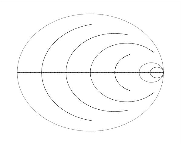
Constant Resistance Circles
 |
| Constant Resistance Circles |
Now the chart gets interesting. From the reflection coefficient equation, we can show\footnote{See notes at the end of the tutorial.} that the radius of each constant resistance circle is
$$r = \frac{1}{A+1}$$
and that the center is at
$$x = \frac{A}{A+1}$$
where \(x\) is the linear value along the \(B=0\) axis, \(-1\) to \(1). These values are shown below.
| A | Center | Radius |
|---|---|---|
| 0 | 0 | 1 |
| 0.2 | 0.166667 | 0.833333 |
| 0.5 | 0.333333 | 0.666667 |
| 1.0 | 0.5 | 0.5 |
| 2.0 | 0.666667 | 0.333333 |
| 5.0 | 0.833333 | 0.166667 |
| 10 | 0.909091 | 0.090909 |
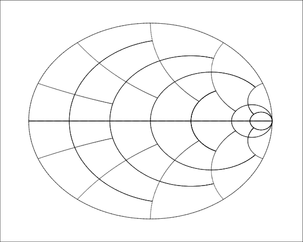
Constant Reactance Circles
 |
| Adding Constant Reactance Circles |
It can also be shown that the center of each constant reactance circle along the \(A=\infty\) axis is
$$y = \frac{1}{B}$$
The radius is
$$r = \left|\frac{1}{B}\right|$$
The centers and radii for the circles are shown in the following table.
| B | Center | Radius |
| -5.0 | -0.2 | 0.2 |
| -2.0 | -0.5 | 0.5 |
| -1.0 | -1.0 | 1.0 |
| -0.5 | -2.0 | 2.0 |
| -0.2 | -5.0 | 5.0 |
| 0.2 | 5.0 | 5.0 |
| 0.5 | 2.0 | 2.0 |
| 1.0 | 1.0 | 1.0 |
| 2.0 | 0.5 | 0.5 |
| 5.0 | 0.2 | 0.2 |
By the way, setting\(A\)equal to zero in the reflection coefficient equation gives the point where the constant reactance and zero resistance circles intersect.
$$\rho = \frac{B^2 + j2B - 1}{B^2 + 1} = -\frac{1-jB}{1+jB}$$
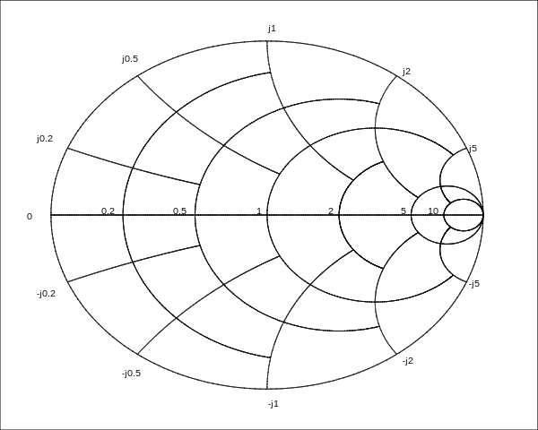
Numbering and Formatting
I like to number the resistance circles along the zero reactance line, and number the reactance circles around the zero resistance circle.
Instead of complete constant resistance circles, I suggest stopping them at strategic points. Since everything on a Smith chart is centered on the right side at \(B=0\), it tends to get a little cluttered there.
 |
| The Decluttered Chart |
To create the chart above, select the desired circle that is being drawn, and then the conjugate circle where it stops. Enter these as A and B.
$$\left(x - \frac{A}{A+1}\right)^2 + y^2 = \left(\frac{1}{A+1}\right)^2$$
$$\left(x - 1\right)^2 + \left(y - \frac{1}{B}\right)^2 = \frac{1}{B^2}$$
Simplifying,
$$y^2 = \left(\frac{1}{A+1}\right)^2 - \left(x - \frac{A}{A+1}\right)^2 \\
>= x^2 - \frac{2A}{A+1}x + \frac{A^2+1}{\left(A+1\right)^2}$$
$$y = x - \frac{\frac{2A}{A+1} \pm \sqrt{\frac{4A^2}{\left(A+1\right)^2}-\frac{4A^2+4}{\left(A+1\right)^2}}}{2} = x - \frac{A\pm2}{A+1}$$
$$x^2 - 2x + 1 + y^2 - \frac{2y}{B} + \frac{1}{B^2} = \frac{1}{B^2} \\
x^2 - 2x + y^2 - \frac{2y}{B} = -1$$
Of course, to draw the chart by hand, simply use the centers and radii found in the tables above.
Notes
Derivation Radius and Position of the Constant Resistance Circles
Setting \(B\) to zero in the reflection coefficient equation gives the point where the right side of the constant resistance circle intersects the zero reactance axis.
$$\rho = \frac{A^2-1}{\left(A+1\right)^2} = \frac{A-1}{A+1}$$
The radius of the circle will be the distance from there to the right side of the zero resistance circle (\(x=1\)).
$$\frac{1 - \left(A - 1\right)/\left(A + 1\right)}{2} = \frac{1}{A+1}$$
And the center will be
$$1 - \frac{1}{A+1} = \frac{A}{A+1}$$
This gives a standard form for the equation of the circles as
$$\left(x - \frac{A}{A+1}\right)^2 + y^2 = \left(\frac{1}{A+1}\right)^2$$
Derivation of the Height of the Constant Reactance Circles
 |
| Constant Reactance Circle Construction |
Right triangle DEF has angle \(\alpha\) at the point where the constant reactance circle intersects the zero resistance circle.
Since sides D and H are parallel, angles \(alpha\) and \(rho\) are equal. This means that triangles DEF and FGH are similar, because they share a side and each have two equal angles (angle-angle-side). Therefore, the ratios of side F to side D for triangle DEF is the same as the ratio of triangle FGH side H to side F. We can express side H in terms of sides F and D
$$H=\frac{F}{D} F = \frac{F^2}{D}$$
From Pythagorean theorem,
$$F=\sqrt{D^2 + E^2}$$
\(E\) is the radius of the zero resistance circle, \(1\) minus the real part of the zero-resistance - constant reactance intersection, \(C\).
This gives us the expression for \(H\).
$$H = \frac{D^2 + \left(1-C\right)^2}{D}$$
\(C\) and \(D\) come from the reflection coefficient equation.
$$H=\frac{\left(\frac{2B}{B^2+1}\right)^2+\left(1-\frac{B^2-1}{B^2+1}\right)^2}{\frac{2B}{B^2+1}}=\frac{4B^2+4}{{2B}\left(B^2+1\right)}=\frac{2}{B}$$
The center and radius of the constant reactance circle will be\(1/2H = 1/B\).
The standard form for the circle becomes
$$\left(x - 1\right)^2 + \left(y - \frac{1}{B}\right)^2 = \frac{1}{B^2}$$
Thursday, July 10, 2014
Silver-Marshall 1929 Plant, 65th Street, Chicago
View Larger Map
In a 1929 Radio News article, there is an architecht's drawing of the plant, built five years after Silver and Marshall started out in a parking garage.
According to Radio News, by 1932 the company only occupied a small portion of the building. An interesting note is that Silver decided (probably with good reason) that Chicago was becoming a radio industry hot spot.
In Audio magazine article "Nothing New Under the AM Sun", Michael N. Stosich notes that EH Scott and Silver-Marshall battled it out for technical supremacy until Silver-Marshall failed in 1940. He goes on to say that McMurdo Silver committed suicide in 1947. Note: Searching Google Maps for the original 6401 W. 65th Street address lands one a couple of blocks east of the correct location.
Saturday, November 03, 2012
A Manufacturer in Indianapolis
A few years ago I found a beautiful marketing sign under the tree at Christmastime. My wife and I both like historical items, and prowl the antique malls when we have an hour or two to ourselves.
The sign adorns my hamshack now.
I had heard of Fairbanks Morse, but only as a manufacturer of industrial equipment - pumps and such. I had no idea they made radios.
It turns out they were located in Indianapolis.
I have added the location to the Radio Row google maps file.
The sign adorns my hamshack now.
I had heard of Fairbanks Morse, but only as a manufacturer of industrial equipment - pumps and such. I had no idea they made radios.
It turns out they were located in Indianapolis.
I have added the location to the Radio Row google maps file.
Monday, August 13, 2012
Radios at the Indiana State Fair
I'm always looking for radio technology in museums and antique malls.
At the Indiana State Fair this year, I wandered through the antiques entries. Among the assortment of All American Fives and an impressive group of early transistor radios I found this beauty.
It appears to be a crystal radio set, with a Bakelite front panel and wooden case.
At the Indiana State Fair this year, I wandered through the antiques entries. Among the assortment of All American Fives and an impressive group of early transistor radios I found this beauty.
It appears to be a crystal radio set, with a Bakelite front panel and wooden case.
Subscribe to:
Posts (Atom)